GLM: posthoc power
0.2.0
Here we compare the results of PAMLj with other software that performs power analysis. In particular, we will compare our results with R pwr package and G*Power.
We use a few examples from G*Power manual, then we test some other design and analysis. In all these example the aim of the analysis is to find the post hoc power given an effect size, a sample size and the design characteristics.
Multiple regression
Multiple Regression - omnibus (deviation of R 2 from zero), fixed model, p. 33
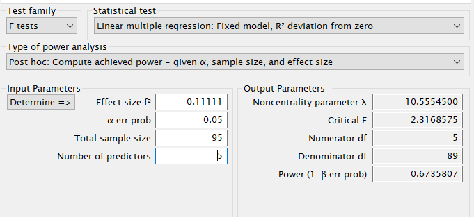
Here we estimate the post-hoc power for the F-test associated to the \(R^2\) of a model with 5 predictors. Five predictors means that the model degrees of freedom are 5. Because the test is on the whole model \(R^2\), also the the effect DF are 5. The \(R^2\) is transformed into the \(f^2\) effect size with the simple formula \(f^2=R^2/(1-R^2)\).
Setup
- Aim = power
- Expected \(R^2\) = .10
- \(f^2\) = 0.1111
- Sample Size (N) = 95
- Effect DF = 5
- Model DF = 5
- Alpha = .05
G*Power
R
In R, we can use the pwr.f2.test command, just plugging
in the effect size \(f^2\) and the
effect DF \(u=5\). However, \(N\) should be inserted as the residuals
degrees of freedom, thus we have \(v=N-u-1=95-5-1=89\)
##
##      Multiple regression power calculation
##
##               u = 5
##               v = 89
##              f2 = 0.1111
##       sig.level = 0.05
##           power = 0.6735347
PAMLj
In PAMLj we can use both Partial Eta-Squared or Eta-Squared, because in the case of the \(R^2\) the two effect size are identical. For simplicity, we use Partial Eta-Squared
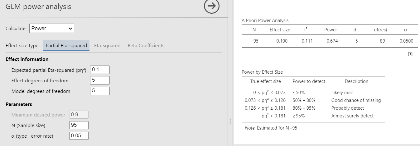
Had we used Eta-Squared, we simply put the \(R^2\) to test both in the effect size and the \(R^2\) field, obtaining the same results.
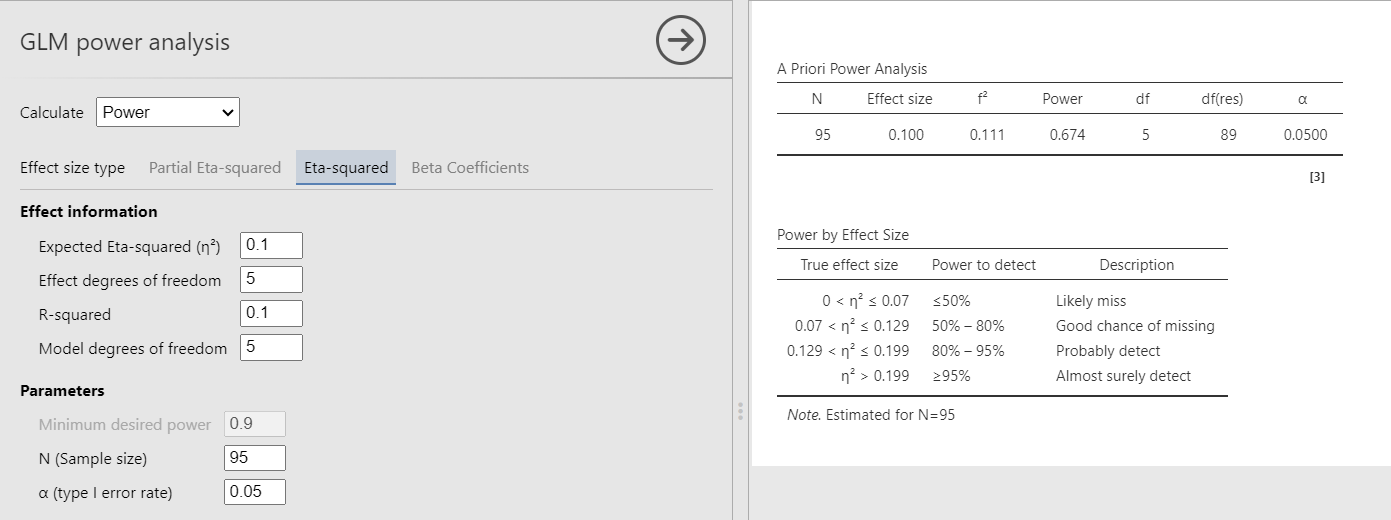
We obtain the same results in packages, although we will see that this is not always the case (see next example).
Increase in \(R^2\)
F test: Multiple Regression - special (increase of R2), fixed model , p. 37
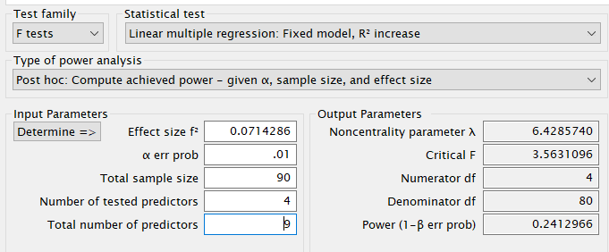
The first example examines a linear model (regression) with \(R_f^2=.30\) with 9 predictors and compare it to a nested model with \(R_n^2=.25\) with 5 predictors. Basically, the test is aimed at testing the variance explained by 4 predictors present in the full model but not the nested model. The variance explained by the 4 predictors is therefore \(R_f^2-R_n^2=.30-.25=.05\). This is also called \(\Delta R^2\), but more formally is a \(\eta^2\) with 4 degrees of freedom evaluated in a model with 9 degrees of freedom.
The \(\eta^2\) is transformed into the \(f^2\) effect size with the simple formula \(f^2=(R_f^2-R_n^2)/(1-R_f^2)\).
Setup
- Aim = power
- \(R_f^2\) = .30
- \(R_n^2\) = .25
- \(\eta^2\) = 0.05
- \(f^2\) = 0.07143
- Sample Size (N) = 90
- Effect DF = 4
- Model DF = 9
- Alpha = .01
G*Power
R
In R, we can use the pwr.f2.test command, just plugging
in the effect size \(f^2\) and the
effect DF \(u=4\). Keeping in mind that
the model has \(m=9\) degrees of
freedom, the \(N\) is inserted as the
residuals degrees of freedom, that is \(v=N-m-1=90-9-1=80\)
##
##      Multiple regression power calculation
##
##               u = 4
##               v = 80
##              f2 = 0.07142857
##       sig.level = 0.01
##           power = 0.2225083
Notice that the results (power) are similar, but not as
close as before. This is because and GPower and
pwr:pwr.f2.test() use two different computations of the
F-distribution non centrality parameter $“. GPower uses
\(\lambda=f^2 \cdot N\), whereas
pwr:pwr.f2.test() uses \(\lambda=f^2 \cdot (u+v+1)\). PAMLj allows to choose which one to use. To
obtain the correct power one should adjust the effect size such that the
non-centrality parameter will be correct. One can do this:
N<-90
u<-4
v=80
f2=.05/(1-.30)
f2adj<-f2*N/(v+u+1)
pwr::pwr.f2.test(f2=f2adj,u=u, v=v,sig.level=.01)
##
## Multiple regression power calculation
##
## u = 4
## v = 80
## f2 = 0.07563025
## sig.level = 0.01
## power = 0.2412965The power is now identical to the one estimated in GPower.
PAMLj
By default, PAMLj employs the GPower non centrality parameter, yielding the same results as GPower.
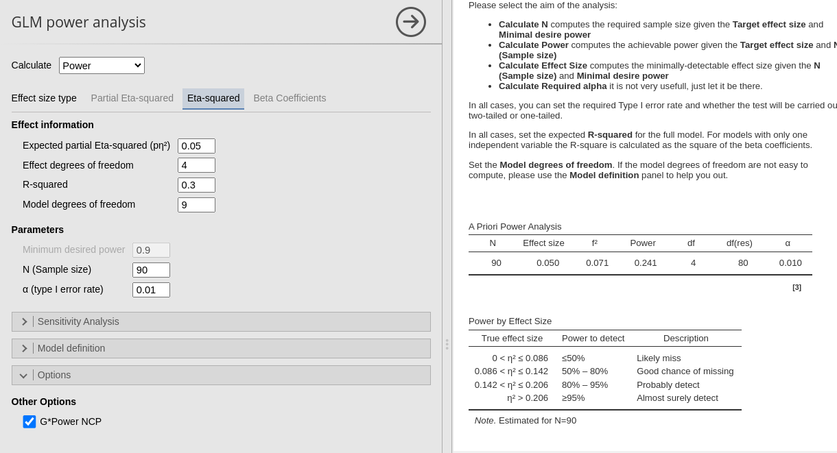
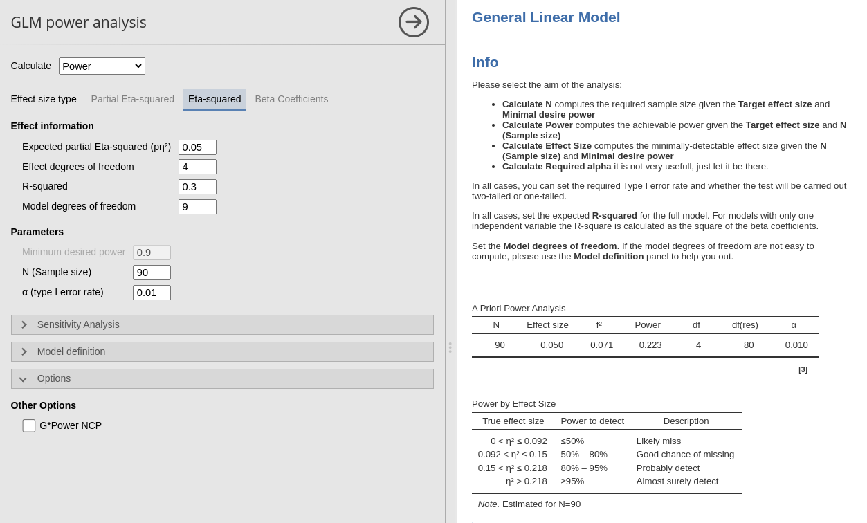
BY de-selecting the option G*Power NCP, we obtain the same results as in R without adjustment.
ANOVA
F test: Fixed effects ANOVA - special, main effects and interaction p. 27
Here we have an ANOVA design \(A \times B \times C\) with \(A\) and \(B\) having 3 levels and \(C\) with 4 levels. Thus the overall model features 36 groups, with \(A\) and \(B\) effects having 2 degrees of freedom, and \(C\) having 3 DF. The researcher is interested in the power of the test associated with the interaction \(A*B\), with a partial Eta-squared \(p\eta^2=0.05665751\) (here the value is slightly different than in GPower manual, but this value honors the f value used in the manual). The interaction will have \(DF=2*2=4\) degrees of freedom, and the whole model will have \(DF=35\), the number of groups minus one. Here are the parameters.
Setup
- Aim = power
- \(p\eta^2\) = 0.05665751
- \(f\) = 0.24507
- Sample Size (N) = 90
- Effect DF = 4
- Model DF = 35
- Alpha = .05
G*Power
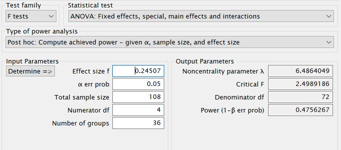
First notice that for this problem, G*Power offers F test: Fixed effects ANOVA routine, which requires an \(f\) as the effect size . \(f\) is simply the square root of \(f^2\) so it can be computed from the partial Eta-squared as \(f=\sqrt{p\eta^2/(1-p\eta^2)}\) .
Plugging in the parameters we obtain:
R
As we have seen before, pwr.f2.test command will
underestimate the power due to the fact that the non centrality
parameter is smaller than the one used in G*Power. Nonetheless, we can
get an estimation of the power by adjusting the effect size \(f^2\) such as to match the correct NCP will
be \(\lambda=Nf^2\). The effect DF
\(u=4\) and the model DF are \(m=35\), yielding \(v=N-m-1=108-35-1=72\)
f<-0.2450722
u<-4
m<-35
N=108
v<-N-m-1
f2<-f^2*N/(u+v+1)
pwr::pwr.f2.test(f2=f2,u=4, v=72,sig.level=.05)
##
## Multiple regression power calculation
##
## u = 4
## v = 72
## f2 = 0.08424054
## sig.level = 0.05
## power = 0.4756346We obtained the same results as in G*Power
PAMLj
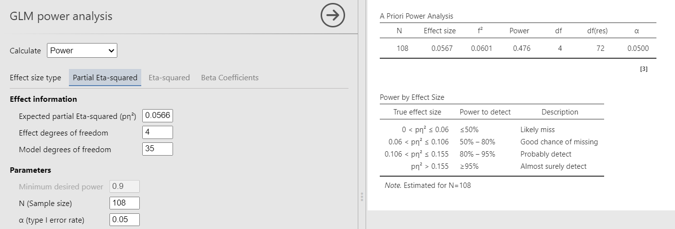
We plug in the partial Eta-squared and the required parameters, and we obtain the same results as before.
Comments?
Got comments, issues or spotted a bug? Please open an issue on PAMLj at github or send me an email