RM-AVOVA

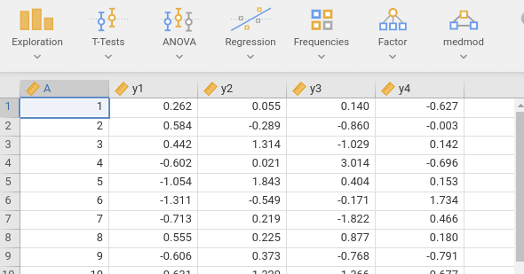
The data mimic a repeated-measures design, with time as a categorical independent variable with four levels and a continuous dependent variable. To analyze them with repeated-measures ANOVA, we require a wide-format dataset, with one row per participant and the following structure:

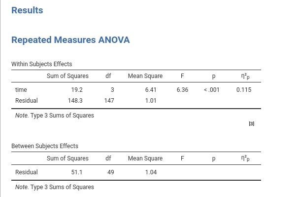
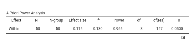
The repeated-measure ANOVA has one categorical variable (time) measured over 4 times. The dependent variable is a continuous variables. Based the RM-ANOVA on a sample of 50 cases, we obtain a partial eta-squared \(\eta_p^2=.115\).

With this information, we estimated the required sample size to obtain a power of at least .90 using PAMLj Factorial Designs command.

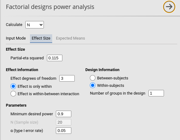
obtaining a sample size of \(N=39\).

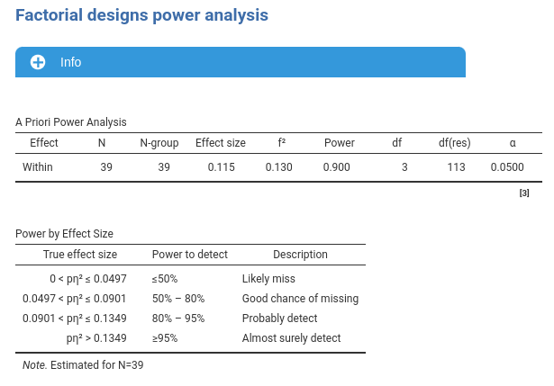
With the original \(N=50\) cases, the expected power would be \(1-\beta=.965\).

Mixed model

The same data, in long format, were analyzed with a mixed model, with time as factor, coded with deviation coding (0’s,-1, and 1’s), and random intercept across participants. Results showed the same F-test of the RM-ANOVA, but give us the coefficients for the contrast variables and the random coefficients variances required to set up the power analysis model.

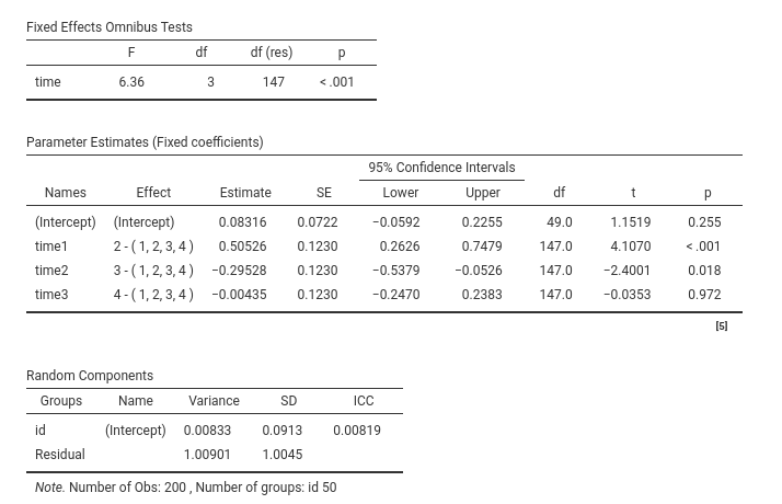
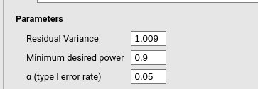
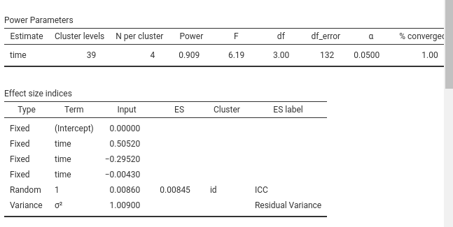
So, the RM-ANOVA results are equivalent to a mixed model with three contrast variables representing time, with coefficients \(.5052\),\(-.2952\), and \(-.0043\). The random intercept variance was \(\sigma_I^2=.0086\) and the residual variance \(\sigma^2=1.009\). We can plug these values in the mixed model power analysis command.

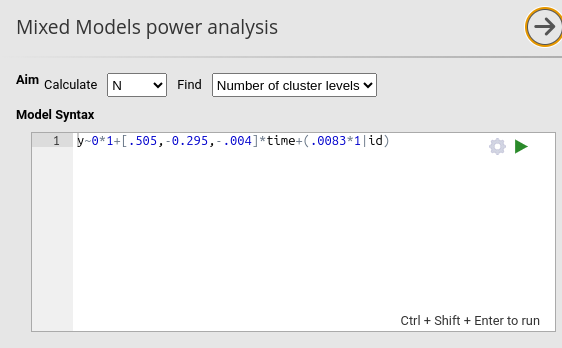
First, we use the squared-brackets syntax to attach three coefficients to the corresponding contrast variables representing time. Second, we multiply the random intercepts (1 in 1|id) by the expected variance (\(.0083\)). This way, we pass the expected coefficients required to build the mixed model for simulating power and finding the required N. Notice that the coefficient for the fixed intercept is set to zero 0*1+... because its value is immaterial for the power computation.

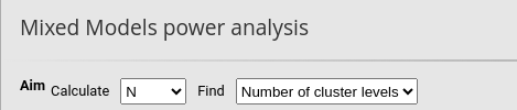
Because in this model participants are the clusters of the model, we set Calculate: N as aim and Number of cluster levels as specific aim.

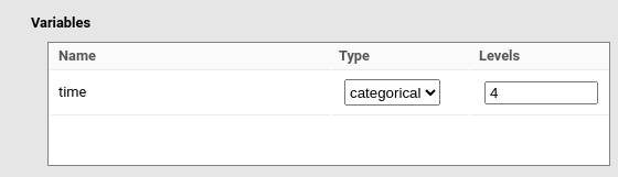
We then specify in the Model Structure -> Clustering variables that the variable id (the participants) has N per cluster equal to 4, because within each participant there will be 4 repeated measures.

Then, we specify that the variable time is a categorical variable with 4 levels.

Finally, we set the residual variance of the model to \(1.009\) as we found in the mixed model.

Running the analysis yield a required N (Cluster levels=number of participants) of 39, as expected by the RM-ANOVA power analysis. Because the mixed model power analysis is based on Monte Carlo simulations, different runs may yield slightly different N, but the results substantially converge.

As an additional check, we compute the expected power of the mixed model test of time based on the original 50 participants. We get \(1-\beta=.966\), remarkably similar to the one obtained with the RM-ANOVA power analysis (\(1-\beta=.966\))

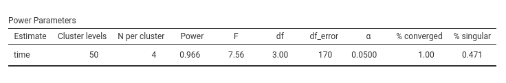
Again, repeating the calculation yields slightly different results, but all substantially congruent with the expected values.

References