Factor Analysis

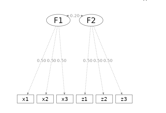
in semPower one can obtain the required N by issue the following command.

library(semPower)

model1<-semPower.powerCFA(type="a-priori", alpha=.05,power=.80,comparison="restricted",
                          loadings=list(
                              c(.5,.5,.5),
                              c(.5,.5,.5)
                          ),
                          Phi=.2,
                          nullEffect= 'cor = 0',
                          plotShow=FALSE
                          )

summary(model1)

## 
##  semPower: A priori power analysis
##                                    
##  F0                        0.010050
##  RMSEA                     0.100251
##  Mc                        0.994987
##                                    
##  df                        1       
##  Required Num Observations 783     
##                                    
##  Critical Chi-Square       3.841459
##  NCP                       7.859363
##  Alpha                     0.050000
##  Beta                      0.199476
##  Power (1 - Beta)          0.800524
##  Implied Alpha/Beta Ratio  0.250657

The same results can be obtained in PAMLj. In the module, we need to specify the model we have in mind, and which parameter is to be tested, that is constrained to zero.

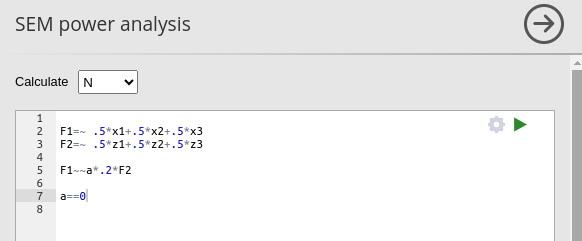
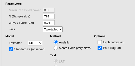
Setting the power parameters as intended

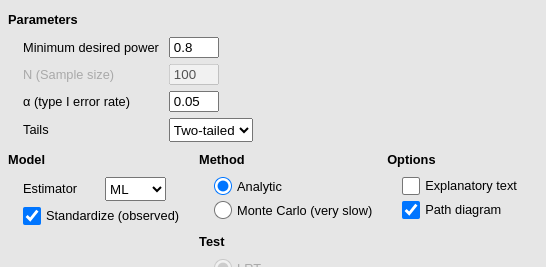
we obtain the same results as before.

We can check now that both packages reaches the same conclusion also if we set \(N=783\) and ask for the expected power.

model2<-semPower.powerCFA(type="post-hoc", alpha=.05,N=783,comparison="restricted",
                          loadings=list(
                              c(.5,.5,.5),
                              c(.5,.5,.5)
                          ),
                          Phi=.2,
                          nullEffect= 'cor = 0',
                          plotShow=FALSE
                          )

summary(model2)

## 
##  semPower: Post hoc power analysis
##                                   
##  F0                       0.010050
##  RMSEA                    0.100251
##  SRMR                     0.032733
##  Mc                       0.994987
##  GFI                      0.996661
##  AGFI                     0.929883
##  CFI                      0.971272
##                                   
##  df                       1       
##  Num Observations         783     
##  NCP                      7.859363
##                                   
##  Critical Chi-Square      3.841459
##  Alpha                    0.050000
##  Beta                     0.199476
##  Power (1 - Beta)         0.800524
##  Implied Alpha/Beta Ratio 0.250657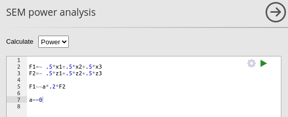

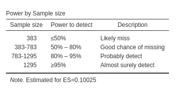
It is useful to verify also the sensitivity analysis table Power by Sample size. We can see that it says that for \(N<383\), we should expect a power less than \(.50\). We can verify this with semPower.

model3<-semPower.powerCFA(type="post-hoc", alpha=.05,N=383,comparison="restricted",
                          loadings=list(
                              c(.5,.5,.5),
                              c(.5,.5,.5)
                          ),
                          Phi=.2,
                          nullEffect= 'cor = 0',
                          plotShow=FALSE
                          )

summary(model3)

## 
##  semPower: Post hoc power analysis
##                                   
##  F0                       0.010050
##  RMSEA                    0.100251
##  SRMR                     0.032733
##  Mc                       0.994987
##  GFI                      0.996661
##  AGFI                     0.929883
##  CFI                      0.971272
##                                   
##  df                       1       
##  Num Observations         383     
##  NCP                      3.839228
##                                   
##  Critical Chi-Square      3.841459
##  Alpha                    0.050000
##  Beta                     0.500183
##  Power (1 - Beta)         0.499817
##  Implied Alpha/Beta Ratio 0.099963

coherently, we obtain a power of \(0.499817\).

Latent variables regression

Let’s now consider a popular model with three latent variables, one common cause of the other two, each measured with some indicators. We consider the PoliticalDemocracy example in (lavaan webpage)[https://lavaan.ugent.be/].

The model looks like this:

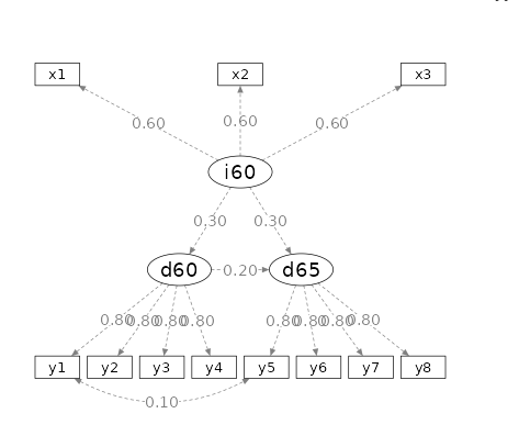
we want to test that at least one effect on dem65 is significant, and obtain the required N to achieve that. This means that we need to constrain both \(dem65=.3*ind60\) and \(dem65=.2*dem60\) to zero. In PAMLj we set the model like this.

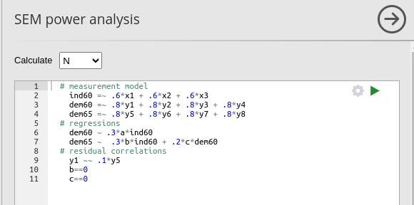
and we obtain

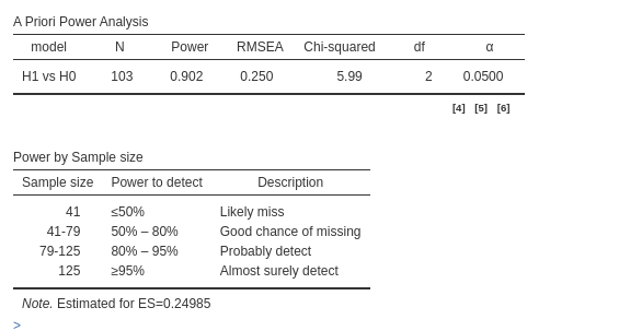
In semPower we can obtain the required power parameters as follows:

popModel<-'

   ind60 =~ .6*x1 + .6*x2 + .6*x3
    dem60 =~ .8*y1 + .8*y2 + .8*y3 + .8*y4
    dem65 =~ .8*y5 + .8*y6 + .8*y7 + .8*y8
  # regressions
    dem60 ~ .3*ind60
    dem65 ~  .3*ind60 + .2*dem60
  # residual correlations
    y1 ~~ .1*y5
'

h1Model<-'

   ind60 =~  x1 + x2 + x3
    dem60 =~ y1 + y2 + y3 + y4
    dem65 =~ y5 + y6 + y7 + y8
  # regressions
    dem60 ~  a*ind60
    dem65 ~   b*ind60 + c*dem60
  # residual correlations
    y1 ~~ y5
'

h0Model<-'

   ind60 =~  x1 + x2 + x3
    dem60 =~ y1 + y2 + y3 + y4
    dem65 =~ y5 + y6 + y7 + y8
  # regressions
    dem60 ~  a*ind60
    dem65 ~  b*ind60 + c*dem60
  # residual correlations
    y1 ~~ y5
    b==0
    c==0
'
model4<-semPower.powerLav("a-priori",modelPop=popModel,
                          modelH0=h0Model, 
                          modelH1=h1Model, 
                          power=.90,alpha=.05,
                          plotShow=FALSE)

summary(model4)

## 
##  semPower: A priori power analysis
##                                    
##  F0                        0.074172
##  RMSEA                     0.192578
##  Mc                        0.963593
##                                    
##  df                        2       
##  Required Num Observations 172     
##                                    
##  Critical Chi-Square       5.991465
##  NCP                       12.68348
##  Alpha                     0.050000
##  Beta                      0.099293
##  Power (1 - Beta)          0.900707
##  Implied Alpha/Beta Ratio  0.503561

#lmod<-lavaan::sem(popModel)
#lavaan::lavInspect(lmod,"cov.lv")
#lavaan::lavInspect(lmod,"cor.lv")

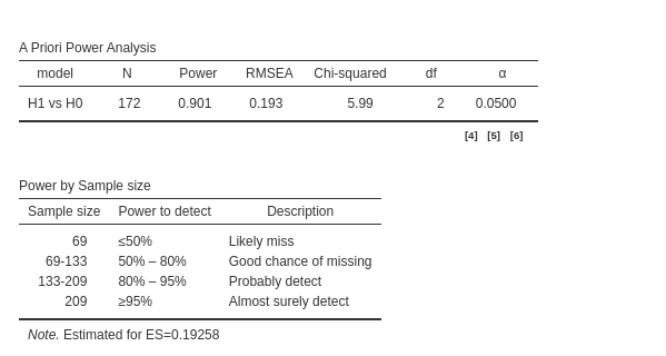
#lavaan::lavInspect(lmod,"std")

This is a remarkable difference! \(N=103\) rather than \(N=172\) is clearly a substantial difference, not just an approximation error. The conundrum is easily explained: PAMLj assumes that all variables, both observed and latent, are completely standardized, while semPower does not. Therefore, in semPower, it is the user’s responsibility to ensure that the scales of the variables are correct.

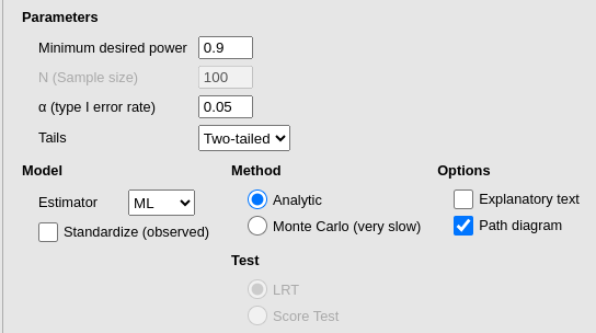
As proof, in PAMLj, we can deselect the option Standardized solution, and we will get exactly the same results as we did in semPower.

However, if the user’s intention is to insert standardized coefficients, the standardized option must be selected. Otherwise, the implied coefficients will differ from the expected ones. To verify this, while keeping the model non-standardized, we can check the Implied Latent Covariances and Standardized regression coefficients in the | Options panel ”

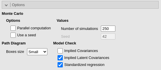
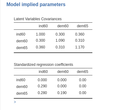
The first table lists the variance-covariance matrix of the latent variables. From the diagonal (variances), it is clear that the latent variables are not standardized. As a result, the Standardized regression coefficients are not the ones we input but a smaller version (in this case). For example, the coefficient from ind60 to dem65 is \(.280\), even though we input \(.30\). These are the actual coefficients implied by the unstandardized model and are the ones used to compute power. This explains why the unstandardized model requires a larger \(N\).

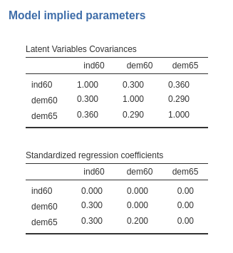
If we standardize the model (with the Standardized solution option selected), the covariances appear correctly standardized, and the regression coefficients are the ones we intended to use.