Mixed models: handling clusters
keywords power analysis, mixed models, multiple clusters, participant by stimuli
0.8.2
Here we discuss some rules for handling clustering variables
(grouping variables) in different designs. We focus on building the
clustering variables in the correct way and checking the results sample
structure, so we set expected power as the aim of the analysis,
and we fill all cluster variables required sizes (#
Cluster Levels and N per cluster).
When the the aim of the analysis is N (with Find being Number of cluster levels
or Cases within clusters), the rules are the same, but one
of size parameter is left empty. It is also a good idea while
experimenting with different designs to set Algorithm to Raw
approximation which is very fast and does not require us to wait
for a simulation to check the resulting sample structure.
One clustering variable
Simple designs with one clustering variable are defined by specifying in Model Syntax the “bars” component of the formula, such as:
y~1*1+1*x+(1*1|cluster)Note
Hereinafter the coefficients are immaterial for our discussion, so we
always set them to 1 and assume random intercepts only. The sample
structure is not altered by the coefficient values or the definition of
fixed and random effects. We also fill in all the cluster size fields:
# Cluster Levels (k) and N per cluster (n). It
is clear that, depending on the aim of the analysis, one of these
parameters will be determined by the algorithm.
PAMLj reads cluster as
the name of the clustering variable and displays the fields to be filled
in to generate the correct sample based on the cluster variable
definition.
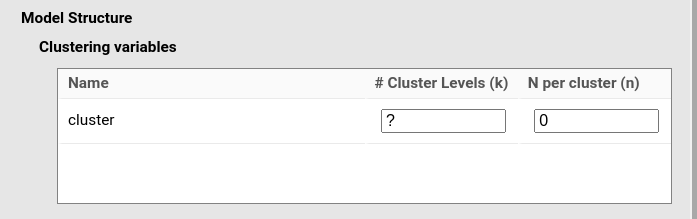
Now, depending on the aim of the analysis, one needs to fill one of
the fields (# Cluster Levels (k) or
N per cluster (n)). Here we discuss the meaning of these
fields, knowing that depending on the goal of the analysis, one of them
will be the target of the power function.
With one clustering variable, # Cluster levels (k) is
the number of groups clustering the observations. In a multilevel
design, say with pupils clustered within classes,
# Cluster levels (k) is the number of classes in the sample
(or the number to be established by the power analysis). In a
repeated-measures design with conditions repeated within participants,
# Cluster levels (k) is the number of participants.
N per cluster (n) is the number of observations within
each cluster level (group). In a multilevel design with pupils clustered
within classes, N per cluster (n) is the (average) number
of pupils in the sample (or the number to be established by the power
analysis). In a repeated-measures design with a condition repeated
within participants, N per cluster is the number of
measurements taken for each participant.
One-way repeated-measures ANOVA design
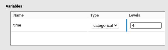
Assume we have a repeated-measures design with four time points (see an example in Mixed vs RM-ANOVA), and one measurement per participant (identified by the variable ID) at each time point. To define this design, we would input:
y~1*1+[1,1,1]*time+(1*1|ID)Then we specify that time is a categorical variable with
4 levels.
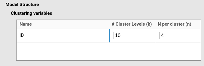
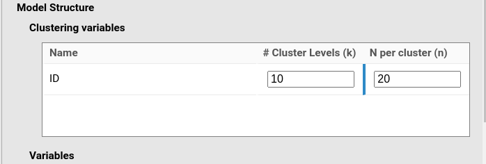
and we set the cluster N per cluster to 4, indicating
that one participant (the cluster unit) has 4 observations (we assume
here we have 10 participants (\(k=10\)), but if the aim is N we would leave
\(k\) empty).
The resulting data look like this:
             y time      ID
1   0.64342217    1       1
2   0.15874249    2       1
3  -0.70961322    3       1
4  -1.46269242    4       1
5  -0.80773575    1       2
6   0.38518147    2       2
7  -1.95162686    3       2
8   2.98249154    4       2
9  -0.04821753    1       3
10 -1.61386528    2       3
11 -0.68877198    3       3
12  1.33885528    4       3
We can see that time is repeated within ID, with one measurement for
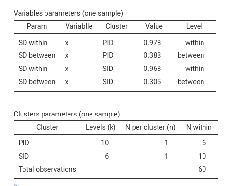
each level of time. Table Variable parameters (one sample)
also shows that we are simulating the correct design, because
time has 4 levels (column Value) repeated within
cluster ID.
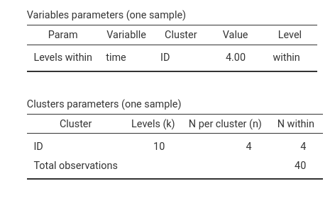
In terms of clusters structure, table Cluster parameters
shows that ID has 10 levels, with 4 observations with each
cluster, and 4 observations within, yielding 40 observations in total.
Whereas in this case the N per cluster (n) and
N within may seem redundant, there are many design
structures in which the two columns conveys different information.
Note
To see the tables reporting on sample charateristics, select the option Variables structure in | Options panel. Clusters structure produces a table with information about the variables and their levels. To see an example of the data generated by your model in PAMLj, select Data structure.
Assume now we have a similar design, but within each time condition the participant is measured 5 times (5 trials). We still have the same model:
y~1*1+1*time+(1*1|ID)and the same variable definition (time with 4 levels), but now
N per cluster is 20, which is 4 levels of time × 5
trials.
The resulting data look like this (first participant):
              y time      ID
1    0.38563267    1       1
2    1.24833377    1       1
3   -0.76549380    1       1
4   -0.94633446    1       1
5    0.72747486    1       1
6   -0.58658441    2       1
7   -1.01631241    2       1
8   -2.66731584    2       1
9    0.62401507    2       1
10   0.15654240    2       1
11  -0.26135861    3       1
12   0.11923442    3       1
13   0.66327673    3       1
14  -0.63811091    3       1
15   0.31462810    3       1
16   0.27796168    4       1
17   0.32836307    4       1
18  -0.34867872    4       1
19  -0.20470434    4       1
20  -0.71480958    4       1
The variable structure is the same as the example above (4 repeated measures), just observations with each participant are now 20 and thus the total number of observation is 200.
Note
Notice that categorical variables are built to vary within clusters by default. This behavior is chosen because in power analysis for mixed model within-cluster variables are more common. However, PAMLj allows to specify between-clusters categorical variables (and also continuous variables). Please read Mixed models: Building factorial designs for help on that.
Multi-cluster designs
Here we discuss cases with more than one clustering variable. When more than one cluster variable is involved, things gets a bit complex (I dare I say wild), but still those designs are doable in PAMLj. One needs a bit more patience to get it right.
Two cases are most relevant for researchers: cross-classified clustering and nested clustering.
Cross-classified clusters
A typical example of cross-classified clustering is an experimental design in which \(P\) participants (identified by the variable PID) are tested with \(S\) stimuli (variable SID). Every participant is exposed to each stimulus, and each stimulus is seen by all participants. We start with the simpler example in which there is only one measurement for each combination of participant and stimulus (a participant sees a stimulus only once).
The mixed model is:
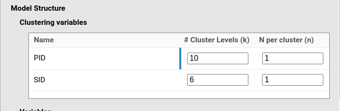
y~1*1+1*x+(1*1|PID)+(1*1|SID)Let’s say we want a sample of 10 participants and 6 stimuli. In total
we have 60 observations, in which each participant has
N per cluster (n) equal to 1, and each stimulus has
N per cluster (n) equal to 1 as well. It may seem counter
intuitive, but the participant is actually repeated only once, but their
measurement is spread across 6 stimuli. Thus, we need to set:
The resulting data (first participant) will look like this:
        y       PID SID
1   0.741008569   1   1
2  -1.001295926   1   2
3   0.728456584   1   3
4   0.649785351   1   4
5  -1.373459856   1   5
6  -2.073459856   1   6
In the Clusters parameters table we can see that we have
6 observations with each participant (PID), because each
participant sees 6 stimuli, and 10 observations within each stimulus,
because each stimulus is seen by 10 participants.
Notice, however, that the independent variable x is continuous, and it is left to vary both across and with clusters by default. For dealing with multiple clusters variables with between vs within independent variables, please see Mixed models: Building factorial designs.
Nested cluster classification
Note
In mixed models estimated following the R package
lme4 syntax, the expression
(1 | school/class) is just a shorthand for specifying
nested random effects. The operator school/class expands
internally into two terms: one random intercept for the grouping factor
school, and one random intercept for the interaction (i.e.,
nesting) school:class. Formally, the random structure
is:
(1 | school) + (1 | school:class)This means that we estimate one random intercept (or whatever random
coefficient we include) per school, and one random intercept per class,
and class are uniquely identified by che combination of school and
class. Accordingly, the Effect size indices table indicates
that the cluster variables are school and
school:class.
The general rule is that, in mixed models, “nesting”
is not a separate statistical concept—it is only a syntactic shortcut.
What matters is the definition of the grouping factors, which in this
example are school and school:class. Random
coefficients (whatever they are) are computed across the groups defined
by these two variables.
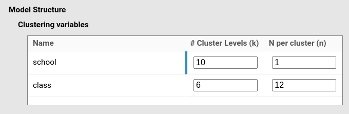
Here things get ugly: Let us consider one of the classic multilevel design: pupils within classes within schools. In this design we have two clustering variables: class and school. In multilevel terminology, pupils are level 0, classes are level 1 with pupils nested within classes, and schools are level 2 with classes nested within schools. To be practical, let us assume we want a sample with 10 schools, each with 6 classes, and each class (on average) with 12 pupils.
First, we set the model:
y~1*1+1*x+(1*1|school/class)Then we specify that we have 10 schools, each with 6 classes, and each class has 12 observations (pupils).
The generated data look similar to the cross-classified data:
row   y             x           school  class
1    0.456717064 -1.017673137      1     1
2   -1.495551991  0.694440645      1     1
3   -0.480543438  0.194002872      1     1
4    0.293003240 -0.116523555      1     1
5   -1.702547420 -1.203825265      1     1
6    1.014035495  0.461345298      1     1
7   -0.415440850 -0.585482460      1     1
8   -1.524924282  0.544323536      1     1
9   -0.106578314 -0.196693360      1     1
10  -0.035543818 -2.741920747      1     1
11   0.229491601  0.170131727      1     1
12  -1.909614050 -1.159812029      1     1
13   1.190966855 -0.356247480      1     2
14  -2.028748115  0.489991721      1     2
15  -1.079830560  1.315918615      1     2
16   0.099924682 -0.330729467      1     2
17  -0.075449795 -2.424778270      1     2
....
However, the estimated model is different as compared with the
cross-classified design. If one looks at the
Clusters parameters table, one finds that the clusters are
now school and school:class, which is exactly
how the model specification expands.
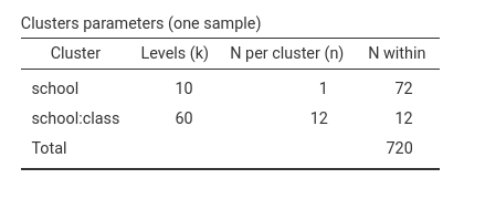
In terms of cluster size, we obtain the results we intended. Let’s check if the setup is correct: each school has 6 classes with 12 pupils, so within each school there are 72 observations. Within each class nested in school there are 12 pupils. But how many observations we’ll have in the sample? Well, 720, because we have 72 observations per school and we have 10 school (\(72 \cdot 10=720\)), or , equivalently, 60 classes with 12 pupils (\(60 \cdot 12=720\)). So, the data are ok.
Apparently nested desings
(Here things remain ugly, and computation gets very slow)
A good rule of thumb in mixed models is that when you are in
doubt about how the clustering variables are related, they are probably
not nested. The second rule is that if nesting (i.e
|cluster1/cluster2) does not come intuitively, things get
clearer if one explicitly thinks in terms of combinations of clusters
levels. The third rule of thumbs is: clusters defined in different
blocks ((1|cluster) being a block) are
cross-classified.
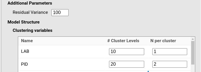
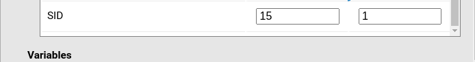
Consider the following design. We have 10 labs (LAB) (or any number you like), each lab conducts an experiment with with 20 participants (PID), each responding to 15 stimuli (SID). Thus, apparently we have a cross-classified experiment nested within labs. What this design actually means is that each level of labs has all 20 X 15 observations corresponding to the cross-classified clustering we have seen above. Thus, we do not have nesting at all, but simply a 3-way classification. Assume the experiment involves a dichotomous factor (cond) with two levels, repeated within-participants. That is, each participant respond to the 15 stimuli in two different conditions.
Now we have to think carefully: we have 10 unique labs, so each labs
requires a random intercept: (1|LAB). Than we have 20
participants for each lab, and each participant is uniquely identified
by being in a particular lab (participant 1 in lab 1 is different than
participant 1 in lab 2): (1|LAB:PID). Stimuli, however, are
not different across labs, because each lab uses the same stimuli. Thus,
we need one random intercept for each stimulus (SID), and they are not
identified by being in a particular labs. Thus: (1|SID)
To set it up, we simply need to specify 3 clustering variable, LABS, PID and SID and their variances in the model.
y~1*1+1*cond+(1*1|LAB)+(1*1|LAB:PID)+(1*1|SID)Now we focus on clusters size. We have 10 labs, each labs is
“measured” once (there is only one experiment per lab). Thus
# Cluster levels=10 and N per cluster=1. We
have 20 participants, each participant sees the stimuli 2 times (one per
condition), so we have # Cluster levels=20 and
N per cluster=2. Finally, we have 15 stimuli, each stimulus
has one replication (one version), so # Cluster levels=15
and N per cluster=1.
This is the resulting sample structure (first rows of the generated dataset):
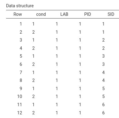
`…
It is clear that each lab has all PID (here not visible) and each
participants sees each stimuli twice, in cond=1 and cond=2. To
appreciate the full sample characteristics we can look at the
Clusters structure table:
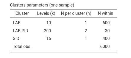
Each participant, identified by the combination LAB:PID
has 30 observations, because it sees 15 stimuli twice. Each stimulus is
seen by 20 participant twice in 10 labs, so each stimulus has 400
observations. Within each lab, however, the experiment implies \(20 \cdot 15\) observations, so each lab has
600 observations. Finally, the 600 observations per lab, summed across
10 labs, yields 6000 observations in total.
Understanding the output design
In all the examples above we set the clusters parameters
(# Cluster Levels (k) and N per cluster (n))
because we focused on understanding how the different parameters yild a
given sample structure. Let’s try now to change the aim of the analysis
to aim:N and Find: Number of cluster levels.
For simplicity, let us assume that we are looking for the minimum number
of labs (LAB) required to obtain a power of at least .90. To
replicate the simulations, let set the Residual
Variance parameter to 500 and use raw approximation
as the finding algorithm.
Running the analysis with these parameters, one obtain (with a small
variability) a Cluster Levels (k) equal to 9. So, given all
the other parameters, we need 9 labs to get at least a power of .90.
Let’s see what the structure of the data is.
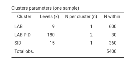
Does it make sense? We need \(9\)
labs, and each experiment requires \(600\) observations. Each participant,
identified by the combination LAB:PID has \(30\) observations, because it sees \(15\) stimuli twice, but now there are \(9\) labs, so the participants are \(20 \cdot 9= 180\), and within each
participant we still have \(30\)
observations as in the previous example. The \(15\) stimuli (SID) are seen by
\(180\) participants twice, so \(180 \cdot 2=360\). Pretty good sense, it
makes.
A variant
What if, however, each labs uses different stimuli. For instant, if
the stimuli are words and different labs conduct the experiment in
different languages, each unique stimulus is identified by the
combination of LAB:SID. Thus, we need to cast this
information in the model. The remaing input definitions are the
same.
y~1*1+1*cond+(1*1|LAB)+(1*1|LAB:PID)+(1*1|LAB:SID)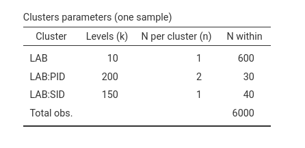
Coherently, we still have 30 observation per participants, that are
200 in total. Each of the 10 labs has 600 observations. Now, however, we
have 150 stimuli (LAB:SID, 15 stimuli for each of the 10
labs), each with 40 observations within (20 participants see each
stimulus twice). The total number of observations are still 6000.
Additional material
Examples
Some worked out practical examples can be found here
Comments?
Got comments, issues or spotted a bug? Please open an issue on PAMLj at github or send me an email